BONUS: Normal Hardy Tour Results

Normally my posts arrive every other Thursday, but I wanted to share a small update regarding a simulation I ran that follows up on a discussion from my last post. I will resume my usual biweekly posts next week.

Recall from the last post that my Smart Hardy simulations of the PGA Tour suggested that, ignoring differences in scoring, average, aggressive, erratic play was a better strategy than conservative, consistent play, in terms of cuts made, wins, and money earned. The post ended with a question: What is the relative importance of scoring average and aggressive strategy? Both factors contribute to better performance, but it would be useful to know how they work in combination. Specifically, it would be interesting to see what happens when consistent players with a low scoring average compete against erratic players with a high scoring average.

It turns out the original Hardy model is an excellent place to start exploring this question. Recall that in the original Hardy model the consistent player had an advantage over the erratic player because he is less likely to hit a bad shot when a normal shot will do. The figure below plots the scoring average for the normal Hardy player as a function of his probability p of hitting an excellent or bad shot.

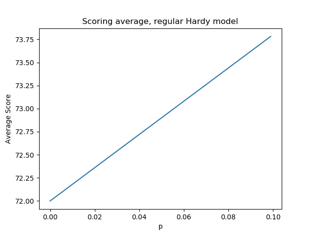
This model sets up exactly the situation of interest. On the one hand, the consistent player has a lower scoring average and will beat the erratic player more often than not. On the other hand, the erratic player is more likely to go really low, which we know generally leads to better performance.

Just as in the Smart Hardy analysis of the last post, I simulated 1 million Tour-style tournaments with normal Hardy players with p values from 0 to 0.1 and counted the number of cuts made, wins, and earnings for each p value.¹ The average results are plotted below.

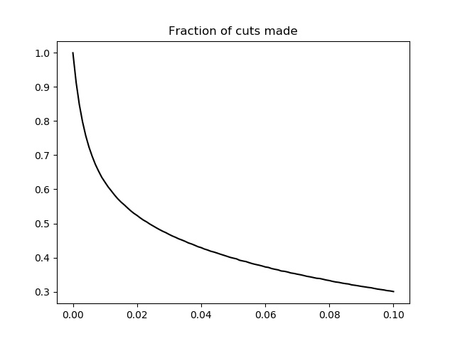
As the figure above shows, the consistent player now has a distinct advantage in making cuts. This is a huge contrast with the Smart Hardy analysis: A player with p=0 in the Smart Hardy model made 0 cuts, but in the normal Hardy model he makes 100% of them! Recall that the reason consistency did not lead to more cuts in the Smart Hardy model was because making the cut required scoring slightly lower than average after two rounds. Since all players in the Smart Hardy model had the same scoring average, it was uncommon for a consistent player to be low enough to make the cut. In contrast, the consistent player’s scoring average in the normal Hardy model is below average, so it is now quite likely that he makes the cut.

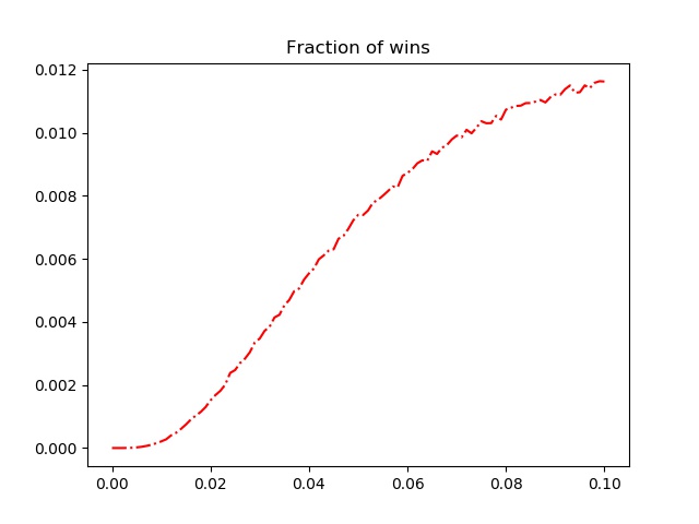
Although the consistent Hardy players are almost certain to make the cut, they almost never win. In fact, the plot of wins vs p above is very similar to the equivalent plot from the Smart Hardy analysis: the higher the p value, the better the chance of winning. The only slight difference is that in this figure the mid-range p values have a slightly higher chance of winning, and the probability of winning appears to level off slightly as p approaches 0.1. Additionally, while the highest probability of winning occurs at p=0.1, the proportion of wins at this value is roughly half the proportion of wins in the Smart Hardy model. It seems that although the erratic player has the highest scoring average, his high variability still gives him the best chance of winning, though the wins are more spread out across p values than they are in the Smart Hardy model.

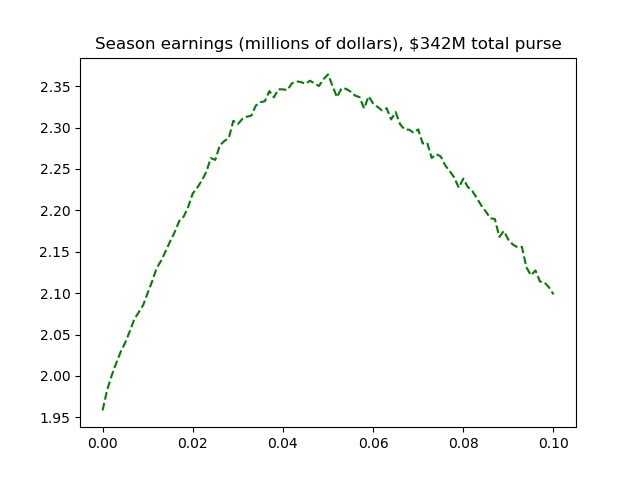
While the consistent player has an edge in making cuts, and the erratic player is most likely to win, the figure above shows the optimal strategy for maximizing earnings seeks to balance these two factors. On the one hand, every cut made leads to a paycheck, so more cuts lead to more individual payments. On the other hand, finishing near the top pays so much better than finishing near the bottom that a single paycheck can make up for a lot of missed cuts. The plot shows that players with a p value near 0.5 maximize their earnings because they make more cuts than the extremely erratic player but also finish higher than the extremely consistent player.

To summarize, these results show that the effects of both a low scoring average and highly erratic play contribute to success in various ways. If Tiger Woods is looking just to maximize his chance of making history, his strategy should be more erratic than a player whose primary goal is to earn the most money possible.

It is worth noting that the plots of wins and season earnings are more noisy than any of the previous plots I have presented. This suggests that in this case 1 million sample tournaments is not enough for the averages to completely converge to their true values. A larger study would likely produce smoother results, but even here the noise is weak enough to clearly identify the overall trend.

It is also important to note that this simulation is just one way to weigh the relative effects of scoring average and variability, and we have no evidence as to what (if any) appropriate weighting would look like. We would expect that if the consistent players had an even better scoring average than the erratic ones (if the slope in the first figure was a lot steeper), the conservative players might have a stronger advantage in winning tournaments and earning more money. Alternatively, we could imagine a distribution of players where the lowest scoring average was near p=0.5, or where both the most consistent and erratic players had the lowest scoring average. There may also be alternative ways to model consistent and erratic play in golf that account for the fact that good shots don’t always save exactly one stroke and bad shots don’t always cost a full stroke.²

Nevertheless, this analysis highlights the complexities presented when both skill and variability are accounted for in a model. It may be worth an increase in scoring average to gain some variability, but the choice depends on a player’s abilities relative to the field and definition of success.